Forecasting by Learning Dynamic External Influence

Introduction

The development of learning algorithms for forecasting events is an important component in building AI systems with a wide range of applications, including in financial markets and healthcare.

Recent progress in these areas has been notable, and methods involving a combination of power sequence models, such as transformers, and elegant probabilistic models, such as temporal point processes, have made enormous progres. However, nearly all existing methods fall short of adequately accounting for or integrating time-varying external factors that influence the outcomes. For instance, stock price variations are affected by a complex interplay of factors that extend beyond mere historical patterns of stock prices. These elements can be shaped by external influences, such as prevailing economic conditions, shifts in governmental policies, and incidents of conflict. Additionally, these factors can be dynamic, with some changing rapidly, others very slowly, some very frequently, and others infrequently.

To study this problem, we develop an approach that captures external influences via temporal Knowledge Graphs (KG) and learns historical patterns via temporal point processes. Considering that such specific temporal KGs are not available in the literature, we develop temporal KGs for financial markets for the machine learning community and propose representation learning techniques to establish benchmark results. The temporal KGs we constructed integrated diverse components, including first and second-order stock relationships, corporate events, macroeconomic indicators, events derived from financial statements, financial ratios disclosed during earnings calls, and analyst sentiments. Notably, all these elements are equipped with time-aware attributes. The capacity to incorporate entities of varying categories, such as Person, Stock Assets, Products, and Alliance, results in an intrinsically heterogeneous knowledge graph. We refer to these KGs as STOCKnowledge aims to encapsulate all pertinent information related to stock assets within a given share market.

Problem Statement

We consider a forecasting problem defined on a multivariate time series \( \mathcal{P} = (\mathcal{P}_i^\tau : i = 1, \dots, N)_\tau \), where \(N\) values are observed at each discrete time point \( \tau_1, \tau_2, \dots \).

At a given time \(T\), our goal is to forecast a future outcome \(Y^{T+\Delta}\) using the historical observations up to time \(T\):

\[ Y^{T+\Delta} = \mathbf{Y}^\Delta \left( (\mathcal{P}_i^\tau)_{1 \le i \le N}^{\tau_1 < \tau \le T} \right) \]

Here, \(Y^{T+\Delta}\) represents a property of the multivariate series at time \(T+\Delta\). In the stock forecasting setting, \(\mathcal{P}_i^\tau\) denotes the price of stock \(i\) at time \(\tau\), and \(Y^{T+\Delta}\) corresponds to the ranking of all stocks based on their future prices.

Beyond historical price movements, real-world forecasting problems are influenced by external events that evolve over time. We model this external information using a temporal knowledge graph.

Each time series element \((\mathcal{P}_i^\tau)_\tau\) is associated with a node in a temporal knowledge graph \(G\). While the time series evolves continuously, the knowledge graph consists of:

• a static component capturing fixed relationships between entities, and
• a dynamic component capturing time-varying events and interactions.

Events in the graph are represented as edges that are valid for specific time periods, depending on the nature of the event.

We extend a standard knowledge graph, which consists of triples \((h, r, t)\), by introducing temporal validity. This results in temporal relations of the form:

\[ (h, r, t, [\tau_s, \tau_e]) \]

where \(h\) and \(t\) are the head and tail entities, \(r\) is the relation type, and \([\tau_s, \tau_e]\) denotes the time interval during which the relation is valid. If a relation holds at a single time step \(\tau\), it is represented as \((h, r, t, [\tau])\).

The complete temporal knowledge graph is defined as a union of subgraphs:

\[ G = G_{\tau_0} \cup \bigcup_{j=1}^{T} G_{\tau_j} \]

where \(G_{\tau_0}\) denotes the static subgraph and each \(G_{\tau_j}\) contains the relations active at time \(\tau_j\).

At time \(T\), the model receives the following input:

\[ X^T = \left( \mathcal{P}_{1 \le i \le N}^{T-W < \tau \le T}, G_{\tau_0}, G_T \right) \]

This input consists of a sliding window of historical prices over the past \(W\) time steps, the static knowledge graph, and the temporal graph snapshot at time \(T\).

Our objective is to learn a representation \(\mathcal{E}(X^T)\) that enables us to compute ranking scores for stocks at a future time \(T+\Delta\):

\[ \hat{Y}^{T+\Delta} = \mathbf{Y}^{\Delta}_{\mathbf{W}_f} \big( \mathcal{E}(X^T) \big) \]

The learned model ranks stocks based on their expected future performance and evaluates them across multiple forecasting horizons using ranking- and return-based metrics.

Temporal Knowledge Graph construction

The construction of the knowledge graphs STOCKnowledge involved data acquired from multiple sources pertaining to the NASDAQ and NSE share markets. Temporal knowledge graphs were constructed for stocks listed in NASDAQ100, S&P500, and NIFTY500, spanning a period of 20 years, from January 01, 2003 to December 30, 2022.

News articles were collected by scraping data from Seeking Alpha (for NASDAQ) and Money Control (for NSE) using the Selenium library in Python. ^{[1] [2]}

A total of 220,645 news articles were collected for NASDAQ and 272,808 for NSE. Each article includes the headline, body text, publication time, associated stock asset, related sector, and taglines. These articles capture corporate events, earnings reports, and analyst and investor sentiments.

A rule-based pattern matching system was used to identify predefined event types from the news content. The extracted events were incorporated into the STOCKnowledge graph with timestamps corresponding to the publication time.

Financial statements of companies listed on NASDAQ and NSE were obtained by scraping Macrotrends and Top Stock Research using Selenium. ^{[3] [4]}

The collected data includes balance sheets, income statements, cash flow statements, and financial ratios. Annual and quarterly trends derived from these statements were modeled as events and incorporated into the knowledge graph as quintuple representations, where the temporal interval spans the corresponding financial year or quarter.

Macroeconomic indicators such as GDP growth, inflation rate, unemployment rate, trade balance, and fiscal deficit provide a snapshot of the overall economic health of a country. These indicators were collected from Macrotrends for both the United States and India.

Trends in macroeconomic indicators were identified as temporal events with intervals defined by the beginning and end of the reported year and incorporated into the STOCKnowledge graphs.

Corporate events such as dividend announcements and stock splits were obtained from Yahoo Finance for both NASDAQ and NSE. These events were represented in the knowledge graph with timestamps corresponding to their occurrence dates.

STOCKnowledge	NASDAQ	NSE
# Triples	7,568	2,736
# Quadruples	52,083	44,399
# Quintuples	310,916	251,551
# Entities	4,911	1,049
# Relations	370,567	298,686
# Entity Types	12	14
# Relation Types	56	53

Inter-stock relationships are categorized into first-order and second-order relationships. A first-order relationship exists when a statement has company i as the subject and company j as the object. A second-order relationship exists when companies share statements with the same object.

For example, Apple and Foxconn participate in different stages of the production of the product iPhone. This relational data was extracted from Wikibase, which stores structured knowledge from Wikipedia.

A curated set of relations was selected, consisting of 6 first-order and 52 second-order relation types, which were filtered and incorporated into the knowledge graph.

Proposed Learning Mechanism

The input to the model at time \(T\) is defined as:

\[ X^T = \{ \mathcal{P}_i^{\tau \in (T-W, T]},\; G_{\tau_0},\; G_T \} \]

Here, \( \mathcal{P}_i^{\tau \in (T-W, T]} \) denotes the historical price window of length \(W\) for stock \(i\) up to time \(T\). The graph \(G_{\tau_0}\) represents the static subgraph of STOCKnowledge, while \(G_T\) captures the temporal positive subgraph at time \(T\). The total number of stocks is denoted by \(N\).

The objective is to learn an encoder \(\mathcal{E}(X^T)\) that produces embeddings for predicting the ranking of stocks at future time steps. The encoder consists of:

• Sequential Embeddings \( \mathcal{E}_s \) for price dynamics,
• Temporal Process Embeddings \( e_{\mathrm{tpp}} \) modeling event dynamics,
• Relational Embeddings \( \mathcal{E}_r \) integrating graph structure.

These components jointly produce embeddings that are passed to a prediction layer to obtain ranking scores at time \(T + \Delta\).

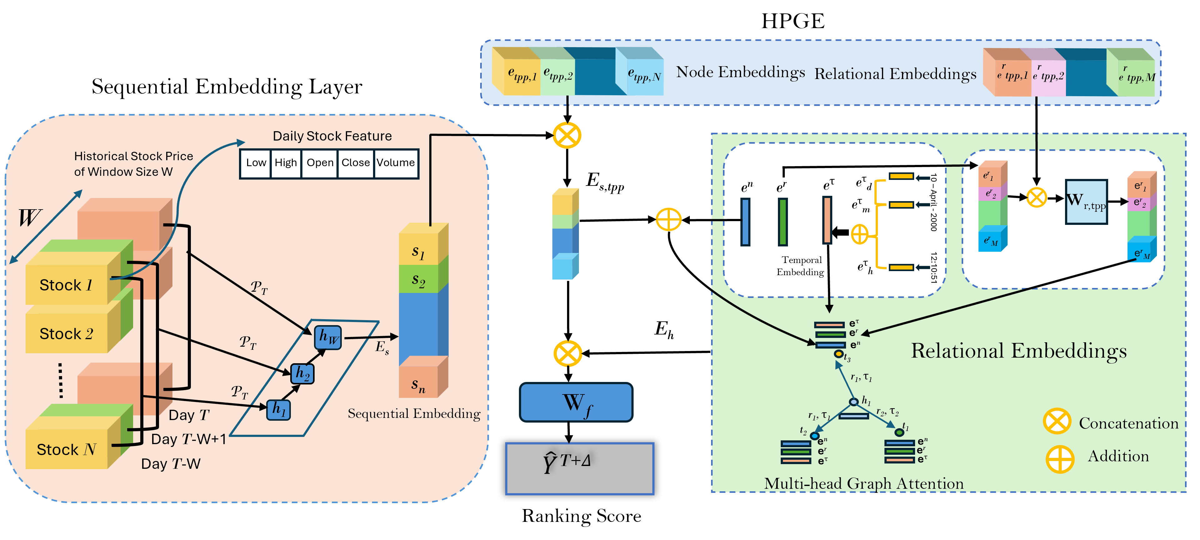
Given the strong temporal dynamics of stock markets, historical price movements play a crucial role in forecasting. We employ a transformer-based sequential encoder to capture long-range dependencies in historical price data and technical indicators.

\[ s_i^T = \mathsf{Transformer}\left( \mathcal{P}_i^T \right) \]

This produces a sequential embedding \(s_i^T\) for each stock \(i\), capturing its temporal behavior over the observation window.

Relations in the dynamic knowledge graph are treated as events in a heterogeneous Hawkes process. For an event \((h, r, t, \tau)\), the conditional intensity function is defined as:

\[ \begin{aligned} \tilde{\lambda}(h, r, t, \tau) &= \mu_r(h, t) + \gamma_1 \sum_{r', t', \tau' \in \mathcal{N}_{<\tau}(h)} m_1(h, r', t', \tau') \\ &\quad + \gamma_2 \sum_{r', h', \tau' \in \mathcal{N}_{<\tau}(t)} m_2(t, r', h', \tau') \end{aligned} \]

Here, \(\mu_r(h, t)\) denotes the relation-specific base intensity, while \(m_1\) and \(m_2\) model mutual excitation effects from historical neighbors.

Node and relation embeddings are initialized as \( e_{\mathrm{tpp}, i} \) and \( e^r_{\mathrm{tpp}, j} \), respectively. The base intensity is parameterized as:

\[ \left\| \sigma\left(\mathbf{W}_e \cdot e_{\mathrm{tpp}, h}\right) + e^r_{\mathrm{tpp}, r} - \sigma\left(\mathbf{W}_e \cdot e_{\mathrm{tpp}, t}\right) \right\|^2 \]

where \(\mathbf{W}_e\) is a dense projection layer and \(\sigma(\cdot)\) is the LeakyReLU activation.

The temporal process embeddings are concatenated with sequential embeddings to form:

\[ E_{s,\mathrm{tpp}} = \left( s_i \,\|\, e_{\mathrm{tpp}, i} \right)_i \]

Each entity \(i\) in the knowledge graph is assigned a learnable embedding \(e^n_i \sim \mathcal{N}(0,1)\). For relation types, embeddings \(e^r_j\) are similarly initialized and concatenated with their corresponding temporal embeddings:

\[ \mathbf{e}^r = \mathbf{W}_{r,\mathrm{tpp}} \cdot \left[ e^r \,\|\, e^r_{\mathrm{tpp}} \right] \]

Temporal embeddings for month, day, and hour are summed to form a unified timestamp embedding \(\mathbf{e}^\tau\). Node embeddings \(\mathbf{e}^n\) and edge attributes \(\mathbf{e}^e = \mathbf{e}^r + \mathbf{e}^\tau\) are passed through heterogeneous graph attention layers to obtain the final relational embedding \(E_h\).

The combined embeddings are passed through a prediction layer to obtain ranking scores:

\[ \hat{Y}^{T+\Delta} = \frac{ \exp\left( \mathbf{W}_f (E_{s,\mathrm{tpp}} \,\|\, E_h) + b_f \right) }{ \sum_{n=1}^{N} \exp\left( \mathbf{W}_f (E_{s,\mathrm{tpp}} \,\|\, E_h) + b_f \right) } \]

These scores define the predicted ranking of stocks based on their expected returns over the horizon \([T, T+\Delta]\).

The overall training objective is defined as:

\[ \begin{aligned} \mathcal{L} &= \alpha_1 \mathcal{L}_1(h, r, t, \tau) + \alpha_2 \mathcal{L}_2(\{\hat{Y}\}, \{Y\}) \\ &\quad + \alpha_3 \mathcal{L}_3(\{\hat{Y}\}, \{D\}) + \alpha_4 \mathcal{L}_4(\{\hat{Y}\}, \{R\}) \end{aligned} \]

The knowledge graph consistency loss is defined as:

\[ \mathcal{L}_1(h, r, t, \tau) = \left\| e^n_h + e^r + e^\tau - e^n_t \right\| \]

The remaining loss terms enforce ranking quality, directional correctness, and emphasis on top-performing stocks.

Publication

Predictive AI with External Knowledge Infusion for Stocks

Code

Our code is available on GitHub.

Authors

• Ambedkar Dukkipati
• Kawin Mayilvaghanan
• Naveen Kumar Pallekonda
• Sai Prakash Hadnoor
• Ranga Shaarad Ayyagari